Category: Statistical Thinking

A fundamental objective of exploring data is to unearth the factors that explain something. For example, does a new drug explain an improvement in a patient’s condition? Does the DNA evidence match the suspect’s? Does the new product feature improve user engagement?

The reigning theory of knowledge, Karl Popper’s critical rationalism, tells us how we cultivate good explanations. Simply put, we start by guessing. We then subject our best guesses to critical tests, aiming to disprove them. Progress emerges from the trial-and-error process of eliminating ideas that fail such tests and preserving those that survive.¹

These guesses, or hypotheses, are not “ultimate truths.” They are tentative, temporary assumptions—like a list of suspects for an unsolved crime.

But how do we objectively evaluate these guesses? Fortunately, statistics provides a solution.

Hypothesis testing is a formal statistical procedure for evaluating the support for our theories. It is hard to understate the huge role this methodology plays in science. It teaches us how to interpret important experimental results and how to avoid deceptive traps, helping us systematically eliminate wrongness.

Feeling insignificant?

Typically with hypothesis testing, we are referring to the null hypothesis significance test, which has been something of a statistical gold standard in science since the early 20th century.

Under this test, a form of “proof by contradiction,” it is not enough that the data be consistent with your theory. The data must be inconsistent with the inverse of your theory—the maligned null hypothesis.

The null is a relentlessly negative theory, which always postulates that there is no effect, relationship, or change (the drug does nothing, the DNA doesn’t match, etc.). It is analogous to the “presumption of innocence” in a criminal trial: a jury ruling of “not guilty” does not prove that the defendant is innocent, just that s/he couldn’t be definitively proven guilty.²

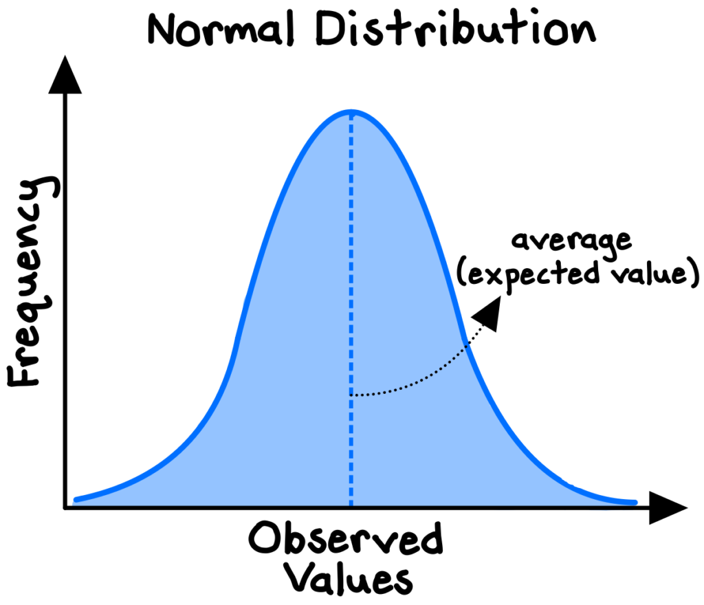
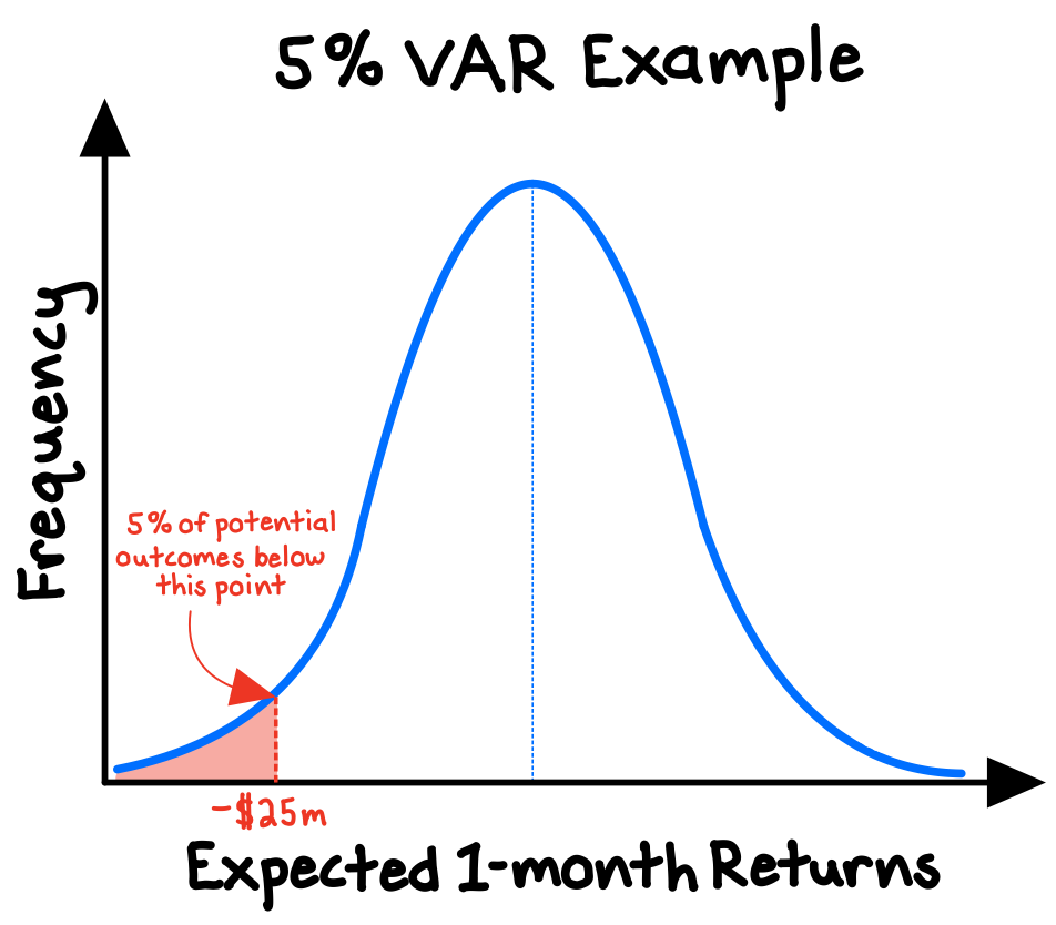
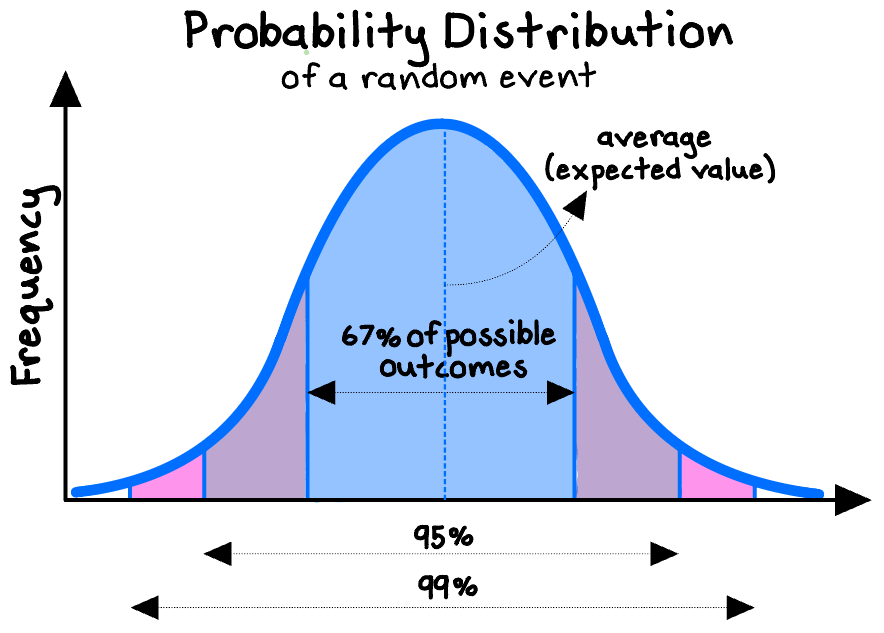
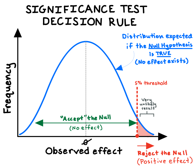
Say we wanted to run a clinical trial to test whether our new drug has a positive effect. We define our null hypothesis as the claim that the drug does nothing, and we plot the expected distribution of those results (the blue bell-shaped curve below). Then, we run an experiment, with a sufficiently large and randomly selected group of subjects, that attempts to refute the null at a certain “significance level”—commonly 5% (see red shaded area below).

The significance level (or “p-value”) represents the probability of observing a result as extreme as we did if the drug actually had no effect—that is, if random variation alone could adequately explain our results. For us to reject the null and claim that our trial provides “statistically significant” support for our drug, we need the observed improvement in our patients’ conditions to be large enough that our p-value very low (below 5%)!

A or B?

We can apply hypothesis testing methods to evaluate experimental results across disciplines, such as whether a government program demonstrated its promised benefits, or whether crime-scene DNA evidence matches the suspect’s.

Essentially all internet-based companies (Twitter, Uber, etc.) use these same principles to conduct “A/B tests” to evaluate new features, designs, or algorithms. Just as with our clinical trial example, the company exposes a random sample of users to the new feature, then compares certain metrics (e.g., click-rate, time spent, purchase amount) to those of a control group that doesn’t receive the feature. Whichever iteration performs best wins. For any app on your phone, its creator likely conducted dozens of A/B tests to determine the combination of features and designs that you see, down to the tempting color of the “Purchase” button!

Stop, in the name of good statistics

Failing to understand hypothesis testing guarantees that we will be wrong more often. Too many people blindly accept faulty or pseudo-scientific experimental results or catchy headlines. They sometimes choose to ignore the science altogether, preferring to craft simple, tidy narratives about cause and effect (often merely confirming their preexisting beliefs).

Even if we do take the time to consider the science, hypothesis testing is far from perfect. Three main points of caution:

1. First, achieving statistical significance is not synonymous with finding the “truth.” All it can tell us is whether the results of a given experiment—with all its potential for random error, unconscious bias, or outright manipulation—are consistent with the null hypothesis, at a certain significance level.
2. Second, significance ≠ importance. To “reject” the null hypothesis is simply to assert that the effect under study is not zero, but the effect could still be very small or not important. For example, our new drug could triple the likelihood of an extreme side effect from, say, 1-in-3 million to 1-in-1 million, but that side effect remains so rare as to be essentially irrelevant.³
3. Third, a significance test, by definition, has only a certain degree of precision which is never 100%. And improbable things happen all the time. For example, a significance level of 5% literally implies a 1-in-20 chance of incorrectly accepting experimental results as true. This enables the nasty “multiple testing” problem, which occurs when researchers perform many significance tests but only report the most significant results. For example, if we do 10 trials of a useless drug with a 5% significance level, the chance of getting at least one statistically significant result gets as high as 40%! You can see the incentive for ambitious researchers—who seek significant results they can publish in prestigious journals—to tinker obsessively to unearth a new “discovery.”⁴

***

Used properly, hypothesis testing is one of the best data-driven methods we have to evaluate hypotheses and quantify our uncertainty. It provides a statistical framework for the “critical tests” that are indispensable to Popper’s trial-and-error process of knowledge creation.

If you have a theory, start by exploring what experiments have been done about it. Review multiple studies if possible to see if the results have been replicated. And if there aren’t any prior research studies, be careful before making strong, unsubstantiated claims. Even better, see if you or your company can perform your own experiment!

The expected value of a process subject to randomness is the average of its outcomes, each weighted by its probability. We might use expected value to evaluate a variety of phenomena, such as the flip of a coin, the price of a stock, the payoff of a lottery ticket, the value of a bet in poker, the cost of a parking ticket, the decision of a business to launch a new product, or the utility of reading a book. The underlying principle of expected value is that the value of a future gain (or loss) should be directly proportional to the chances of getting it.

The concept originated from Pascal and Fermat’s solution in 1654 to the centuries-old “problem of points,” which sought to divide the stakes in a fair way between two players who have ended their game before it’s properly finished. Instead of focusing on what had already happened in the game, they focused on the relevant probabilities if the game were to continue. Their findings laid the foundations for modern probability theory, which has broad applications today, including in statistics (the mean of a normal distribution is the expected value), decision theory (utility-maximization and decision trees), machine learning algorithms, finance and valuation (net present value), physics (the center of mass concept), risk assessment, and quantum mechanics.

Expected value is one of the simplest tools we can use to improve our decision making: multiply the probability of gain times the size of potential gain, then subtract the probability of loss times the size of potential loss.

Simply put, we should bias towards making decisions with positive expected values, while avoiding decisions with negative ones. The idea is that, over the long run, we will be better off if we repeatedly select the alternatives with the highest expected values.

Useful but used wrongly

Lotteries are a classic example. We might genuinely enjoy playing the lottery. But we can’t ignore that lottery tickets are typically really bad bets, even when the jackpot is huge. Because the state takes a cut of the total pot and only pays out the remainder to winners, the expected value for all players must be negative.¹

The expected value rule of thumb may seem straightforward, but a body of fascinating psychological research—particularly the work of Daniel Kahneman and Amos Tversky on “prospect theory”—shows that the decision weights that people assign to outcomes systematically differ from the actual probabilities of those outcomes.

For one, we tend to overweight extreme (low-probability) outcomes (the “possibility effect”). As a result, we overvalue small possibilities, increasing the attractiveness of lotteries and insurance policies. Second, we give too little weight to outcomes that are almost certain (the “certainty effect”). For example, we weigh the improvement from a 95% to 100% chance much more highly than the improvement from, say, 50% to 55%.²

Process over outcome

The expected value model reminds us to be more critical of the process (how we value the possibilities) than the outcome (what we actually get). When randomness and uncertainty are involved—as they almost always are in complex systems—even our best predictions will be wrong sometimes. We can’t perfectly anticipate or control such outcomes, but we can be rigorous with our preparation and analysis.

Remember, too, that expected value doesn’t represent what we literally expect to happen, but rather what we might expect to happen on average if the same decision were to be repeated many times (a better name might have been “average value”). Often we don’t and can’t know the exact expected value, but we can say with some confidence whether it’s positive or negative.⁴

Seeking the “long tail”

In some circumstances, applying expected values may be an entirely misguided approach. We must consider carefully the distribution of the underlying data. For a standard, normally distributed system (e.g., human height, SAT scores), the expected value is also the central tendency of the data, and is therefore a reasonable guess for any individual observation.

However, for power-law distributed systems (e.g., the frequency of words in the English language, the populations of cities), there are a small number of inputs that account for a highly disproportionate share of the output, skewing the distribution of the data. Because power laws are asymmetrical distributions, the expected value is not the central tendency of the data; a few extreme observations wildly skew the results.

Consider the early-stage venture capital industry, in which investors put money into highly risky startup ventures. Financial returns on venture capital investments are power-law distributed. Most of these startups will fail, but the ones that do succeed can really succeed and generate massive financial returns (think Google or Tesla). Thus, for venture capitalists, the game is not to seek the average return or “expected value,” but rather to search for the “long tail”—the extreme outliers that generate outsized results.

Expected value is a lot less relevant when you don’t care as much about the probability of success than you do about the magnitude of success, if achieved. If one or two “grand slams” can generate massive returns for the fund, then VCs don’t care if 90% of their other investments fail.

Union Square Ventures, for example, invested in Coinbase in 2013 at a share price of about $0.20, and realized a massive return when Coinbase opened its initial public offering at $381 in 2021—a valuation of around $100bn and an increase of over 4,000x from the round that Union Square led eight years earlier.⁵

***

Expected value helps us evaluate alternatives even when we face substantial uncertainty our risk. Estimate the potential “payoffs” and weight them by their respective probabilities. In general, err towards making bets with positive expected values, while declining bets with negative ones.

While extremely useful as a rule of thumb, applying expected value can involve substantial subjectivity—and is therefore at risk of bias and error. Use ranges instead of single values to avoid false-precision. And remember that expected value may be entirely inappropriate when dealing with power-law distributed systems, where its not the “middle” outcome that dominates, but the “extreme” ones.

Regression to the mean is the statistical rule that in any complex process that involves some amount of randomness, extreme observations will tend to be followed by more “mediocre” observations.

Although regression to the mean is not a natural law but a statistical tendency, it is an extremely useful mental model, because we have a problematic tendency to get regression wrong. For one, we fail to appreciate its power to explain many apparent phenomena that are really just mirages of randomness. We also often foolishly “predict” regression when what we’ve been observing recently seems extreme.

Innate or random?

It is not some mediocrity-loving law that causes regression to the mean; rather, regression is the natural tendency when inherent characteristics are intermingled with chance. While we should expect inherent traits to show up repeatedly, chance is fleeting.

Consider a clinical trial where we use random sampling to test a new dieting method on overweight folks. Because our body weight fluctuates daily, there is some randomness involved. At initial weigh-ins, the individuals in the heaviest segment are certainly more likely to have a consistent weight problem (an inherent characteristic), but they are also more likely to have been at the top of their weight range on the day you happen to weigh them (a random fluctuation). Therefore, we should expect our heaviest participants to lose some weight on average during the study, regardless of the effectiveness of the diet!¹

Causal mirages

The same logic can be applied to outperforming businesses, artistic success, or sports achievement: all of these success cases are more likely to possess superior talent, but also to have had some luck—and luck, by definition, tends to be transitory.

In assessing cause and effect, we commonly attribute causality to a particular policy or treatment when the change in the extreme groups would be expected without the treatment. Regression does not have a causal explanation. It inevitably occurs when the correlation between two elements (such as body weight and a dieting method) is less than perfect—in other words, whenever some amount of randomness is involved.²

In statistical science, the prescription for this causality error lies in introducing a “control group,” which should experience regression effects regardless of treatment. In our dieting study, we would need to compare the results of the dieting group with those of a group who knows nothing of the diet. We then assess whether the outcomes between the control and treatment groups are more different than regression alone can explain.

In everyday life, we must be prudent before assigning causality to some factor when we observe more moderate outcomes following an extreme one. It’s rather tempting to come up with a coherent narrative about what caused a change than to say, “It’s just statistics.” If we believe strings of good or bad results represent a persistent state of affairs, then we will incorrectly label the reversion to normal as the consequence of some other change we made or observed.³

For example, we could come up with stories such as:

• The saleswoman who generated record sales last year but did worse this year must have become less motivated after she got a big bonus.
• The stock market rebound after last year’s recession means the President’s economic policies must be working.
• When I gave my daughter ice cream after she earned an “A+” on a test, she did worse the next time. But when I sternly criticized her after she got a “C,” she did better the next time. Therefore, I should be more forceful.

In all of these examples, it’s possible that the moderation in behavior we observed could be entirely explained by the basic statistical workings of regression to the mean, regardless of the “causal” story we came up with.

An insane example is the purported “discovery” in the 1976 British Medical Journal that bran had an extraordinary balancing effect on digestion. Subjects with a speedy digestion tended to slow down, those with typical digestion speed were unchanged, and those with slow digestion tended to accelerate. The crazy thing is: due to regression to mean, these are exactly the results we should expect to see if the bran had no effect whatsoever!⁴

***

People tend to prophesy “regression!” after anything extreme happens, without properly understanding why and how it works. Nothing is ever “due” for regression (not the stockmarket, not your football team, etc.). Extreme behavior simply tends not to persist over large samples. Once we understand that the tendency towards mediocrity is inevitable whenever randomness is involved, we can avoid the delusions of causality that plague so many others—whether in business, sports, the stock market, or our weight-loss regimen.

The probability distribution of a random variable defined by a standard bell-shaped curve is known as the normal distribution, which has a meaningful central average (or “mean”) and increasingly rare deviations from the mean. It is a symmetrical distribution in which we expect any random observation to be equally like to fall below or above the average.

Many variables in the real world are normally distributed, or approximately so. A few well-known examples include human height, birth weight, bone density, cognitive skill, job satisfaction, and SAT scores.¹

The normal distribution is one of the most powerful statistical concepts to understand, as the properties of normally distributed processes can be modeled and analyzed with well-established statistical methods and readily available software. These tools allow us to make judgments, inferences, and predictions based on data and to quantify the risk around our hypotheses.

If we are not careful, however, the normal model can lead us into grave errors (including the 2008 financial crisis, which we will explore). But first, we should note that although normally distributed phenomena are common in nature, many processes, especially those taking place in complex systems (such as economies), follow distinctly non-normal distributions and often feature a long right-hand “tail” (such as the distribution of individual incomes). We cannot just blindly use the normal model without understanding the distribution of the underlying data and adjusting if necessary.²

However, that is not the full story.

Bells on bells on bells

The normal model is not, in fact, limited to use only with underlying data that is normally distributed.

Consider a set of source data of 1,000 flips of a coin, where heads and tails each occurred exactly 500 times (as we would expect from a fair coin). This data is clearly not normally distributed (see below). So, are the typical statistical tools useless?

The answer is no.

To see why, let’s take a random sample of, say, 100 flips from the source data, and calculate the fraction of flips that are heads (the sample mean). We expect this percentage to be 50% because that is the population mean of the source data, but, of course, there will be random variation in our sample such that not every sample mean will be exactly 50%.

If we continue to take random samples of 100 flips—say, 500 such samples—and plot the distribution of all the sample means, the distribution of the sample averages will be approximately normal, even though the underlying population data is not normal! This phenomenon is known as the central limit theorem.

Incredibly powerful in statistics, this maxim explains why bell-shaped distributions are so useful, even though source data sets are rarely perfectly normally distributed: the sample means of just about any process subject to some degree of randomness are eventually normally distributed. This occurs because observed data often represent the accumulation of many small factors, such as how our physical traits (e.g., height, birth weight) emerge from the results of millions of random “copy” operations from our parents’ DNA.³

The central limit theorem enables a wide range of statistical analysis and inference, allowing us to ground our decision making in a solid mathematical foundation.

A truly significant bell

The twin tools of random sampling and statistical analysis using the normal model are widely used and remarkably handy.

Perhaps most significantly, the normal distribution lies at the heart of the scientific method. Because we expect that the observed effects in, say, a clinical trial for a new drug (or any scientific experiment) will tend towards a normal distribution, we can assess how “significant” our observed results are by estimating the probability of observing an outcome that extreme if our drug actually had no effect (the “p-value”). If the normal model tells us that the p-value is very low (say, below 5%), then our trial provides statistically significant support for the drug’s effectiveness.

Manufacturers and engineers use the normal model to set control limits for evaluating some measure of system performance. Observations falling outside the control limits alert the system owner that there could be a problem, since we should expect, under the normal model, that such extreme observations are exceedingly unlikely if the system were functioning normally. We should be thankful that these types of controls exist whenever we board a plane or buy a car.

The normal model should also ring a bell (pun intended…) every time we see the results of a political poll. Attached to the headline poll result should be a “margin of error” which describes the amount of potential error expected around those results, given that random sampling involves variation that follows a normal distribution. For example, a poll might show that the Republican candidate has 48% support in polls, with a margin of error of plus-or-minus 3%, implying the “true” value could be anywhere between 45% to 51%.⁴

2008 was not normal

Financial institutions and regulators rely heavily on applications of the normal distribution through value at risk (“VAR”) models, which they use to quantify financial risk exposure, establish tolerable risk levels, and assess whether there is cause for alarm.

VAR models provide an estimate of the minimum financial losses that should be expected to occur some percentage of the time over a certain time period. For example, an investment firm might estimate that, given an assumed (normal) distribution of their portfolio’s potential returns over the next month, they should expect a 5% probability that they will suffer losses of at least $25m (the “value at risk”).⁵

The VAR is simply a point on the (assumed) probability distribution of potential returns for a portfolio. The more radical the deviation from today’s conditions, the lower the probability of that outcome—as the normal model would suggest.

VAR supplies a simple, single risk metric that is widely accepted by leading institutions. However, the VAR model also provides an excellent example of the limitations of the normal model—an indeed of models more generally.

Drawing from historical data, the VAR makes strong assumptions about potential future returns, assumptions which are susceptible to error, bias, and manipulation. Moreover, VAR’s use of a normal distribution makes it inadequate for capturing risks of extreme magnitude but low probability, such as unprecedented asset price bubbles or the collapse of the national housing market.

In the aftermath of the 2008 financial crisis, the U.S. House of Representatives concluded that rampant misuse of the VAR model by financial institutions justified excessive risk-taking, which led to hundreds of billions in losses and helped fuel a global recession.⁶

***

Fluency with basic statistical tools such as the normal model can provide us a valuable edge in our decision-making. It can help us interpret experimental results and political polls, implement quality and safety standards, and quantify financial risks.

But the normal distribution, like all models, is a flawed simplification. It cannot give us certain truth, only suggestions and approximations based on layers of assumptions and theory. Equally important to knowing how to use the normal model is knowing how to determine whether it is appropriate to use in the first place!

The Law of Large Numbers is a theorem from probability theory which states that in normally distributed systems, as we observe more instances of a random event, the actual outcomes will converge on the expected outcomes. In other words, when our sample sizes grow sufficiently large, the results will settle down to fixed averages.

The Law of Large Numbers, unsurprisingly, does not apply to small numbers. The smaller the sample size, the greater the variation in the results, and the less informative those results are. Flipping a coin and observing 80% “heads” in 10 flips is much less remarkable than observing the same imbalance in 10,000 flips (we would start to question the coin). Larger samples reduce variability, providing more reliable and accurate results.

Delusions of causality

Sadly, people tend to be inadequately sensitive to sample size. We focus on the coherence of the story we can tell with the information available, rather than on the reliability of the results. Following our intuition, we are likely to incorrectly assign causality to events that are, really, just random.

Psychologist Daniel Kahneman famously cites a study showing that the counties in the U.S. in which kidney cancer rates are lowest are mostly small, rural, and located in traditionally Republican states. Though these factors invite all sorts of creative stories to explain them, they have no causal impact on kidney cancer. The real explanation is simply the Law of Large Numbers: extreme outcomes (such as very high or very low cancer rates) are more likely to be found in small samples (such as sparsely populated counties).¹

We often foolishly view chance as a self-correcting process. For instance, we might believe that several consecutive successes (in blackjack, basketball, business, etc.) make the next outcome more likely to be a success (the “hot-hand” fallacy). Or, we might believe that a random deviation in one direction “induces” an opposite deviation in order to “balance out” (the gambler’s fallacy).

In reality, the Law of Large Numbers works not by “balancing out” or “correcting” what has already happened, but simply by diluting what has already happened with new data, until the original data becomes negligible as a proportion.² For instance, as we flip a fair coin more and more times, the proportion of flips that land as “heads” will settle down towards 50%.

This is the logic behind the powerful Central Limit Theorem. Essentially no matter what the shape of the population distribution, for larger samples the average can be assumed to be drawn from a normal “bell-shaped” curve. This theorem provides the foundation for all sorts of statistical tests that help us make better inferences and to quantify uncertainty.³

Correlated errors, and why polls can mislead us

A key limitation of the Law of Large Numbers is that the theorem also requires an assumption that the observations we make are independent of one another (for instance, one coin flip does not impact the next). But if the observations are correlated—as they often are in real life—then what appear to be random results could actually reflect a bias in the method.⁴ If our data is systemically biased, we are likely to make errors, and we cannot expect the Law of Large Numbers to work like normal.

The potential for correlation between sampling errors was one of statistician Nate Silver’s key insights when he assigned a much higher probability of a Trump victory in 2016 than other pundits estimated. Based on polling data, Hillary Clinton was favored in five key swing states, and analysts surmised that Trump was extremely unlikely to win all of them, and thus extremely unlikely to win the election. Sure, they assumed, Trump might pull off an upset win in one or two of those states, but the Law of Large Numbers should take over at some point.

Silver, however, recognizing that our entire polling methodology could be systematically biased toward one candidate, modeled a healthy amount of correlation between the state polls. His model implied that Trump sweeping the swing states was way more likely than we would expect from the individual probabilities, because a discrepancy between the polls and the results in one state could mean that we should expect similar errors in the other states. Trump won all five of those states, and won the election.⁵

***

Overall, the Law of Large Numbers demonstrates the incredible danger of relying on small samples to make inferences, the fallacies of assuming that random things are “streaky” or that extreme results will promptly be “balanced out,” and the importance of checking our data for systemic bias—which will lead to misleading results regardless of sample size.

Bayesian reasoning is a structured approach to incorporating probabilistic thinking into our decision making. It requires two key steps:

1. Obtain informed preexisting beliefs (“priors”) about the likelihood of some phenomena, such as a suspect’s DNA matching the crime scene evidence, a candidate winning an election, or an X-ray revealing a tumor.
2. Update our probability estimates mathematically when we encounter new, relevant information, such as finding DNA from a new suspect, a new poll revealing shifting voter behavior, or a new X-ray showing unexpected results.

The Bayesian approach allows us to use probabilities to represent our personal ignorance and uncertainty. As we gather more good information, we can reduce uncertainty and make better predictions.

Unfortunately, when we receive new information, we tend to either (a) dismiss it because it conflicts with our prior beliefs (confirmation bias) or (b) overweight it because we can recall it more easily (the availability heuristic). Bayesian reasoning demands a balancing act to avoid these extremes: we must continuously revise our beliefs as we receive fresh data, but our pre-existing knowledge—and even our judgment—is central to changing our minds correctly. The data doesn’t speak for itself. ¹

The Bayesian approach rests on an elegant but computationally intensive theorem for combining probabilities. Fortunately, we don’t always need to be able to crunch probability calculations, because Bayesian reasoning is extremely useful as a rule of thumb: good predictions tend to come from appropriately combining prior knowledge with new information.

However, as we will see, Bayes is simultaneously super nifty and incredibly limited—as all rules of thumb are.

Why your Instagram ads are so creepy

We experience Bayesian models constantly in today’s digital world. Ever wondered why your Instagram ads seem scarily accurate? The predictive models used by social media apps are powerful Bayesian machines.

As you scroll to a potential ad slot, Instagram’s ad engine makes a baseline prediction about which ad you’re most likely to engage with, based on its “priors” of your demographic data, browsing history, past engagement with similar ads, etc. Depending on how/whether you engage with the ad, the ad targeting algorithm updates its future predictions about which ads you’re likely to interact with.² This iterative process is the reason why your ads seem creepy: they become remarkably accurate over time through constant Bayesian fine-tuning.

Prioritize priors

For Bayesians, few things are more important than having good priors, or “base rates,” to use a a starting point—such as the demographic or historical-usage data on your Instagram account.

In practice, we tend to underweight or neglect base rates altogether when we receive case-specific information about an issue. For example, would you assume that a random reader of The New York Times is more likely to have a PhD, or to have no college degree? Though Times readers are indeed likely to be more educated, the counterintuitive truth is that far fewer readers have a PhD, because the base rate is much lower!³ There are over 20x more Americans with no college degree than those with a doctorate.

The prescription to this error (called “base-rate neglect”) requires anchoring our judgments on credible base rates, and thinking critically about how much weight to assign to new information. Without any useful new information (or with worthless information), Bayes provides us clear guidance: hold to the base rates.

“Pizza-gate”

Many bad ideas come from neglecting base rates.

Consider conspiracy theories, which, despite their flimsy core claims, propagate by including a sort of Bayesian “protective coating” which discourages believers from updating their beliefs when new information inevitably contradicts the theory.

For example, proponents of the “Pizza-gate” conspiracy falsely claimed in 2016 that presidential candidate Hillary Clinton was running a child sex-trafficking ring out of a pizzeria in Washington, DC. A good Bayesian would assign a very low baseline probability to this theory, based on the prior belief that such operations are exceedingly rare—especially for a lifelong public servant in such an implausible location.

When the evidence inevitably contradicts or fails to support such a ludicrous theory, we should give even less credence to it. That is why Pizza-gate proponents, like many conspiracy theorists, introduced a second, equally baseless theory: that a vast political-media conspiracy exists to cover up the truth! The probability of this second theory is also really low, but it doesn’t matter.⁴ With this “protective layer” of a political-media cover-up, conspiracy theorists can quickly dismiss all the information that doesn’t support the theory that Hillary Clinton must be a pedophilic mastermind.

Bayesian reasoning is only as good as the priors it starts with, and the willingness of its users to objectively integrate new, valid information.

The boundaries of Bayes

The mathematics of Bayes’ theorem itself is uncontroversial. But Bayesian reasoning becomes problematic when we treat it as anything more than a “rule of thumb” that’s useful when we have a comprehensive understanding of the problem and very good data.

Estimating prior probabilities involves substantial guesswork, which opens the door for subjectivity and error to creep in. We could ignore alternative explanations for the evidence, which is likely to lead us to simply confirm what we already believe. Or, we could assign probabilities to things that may not even exist, such as the Greek gods or the multiverse.⁵

The biggest problem: Bayes cannot possibly create new explanations. All it can do is assign probabilities to our existing ideas, given our current (incomplete) knowledge. It cannot generate novel guesses. But sometimes, the best explanation is one that has not yet been considered. Indeed, creating new theories is the purpose of science. Scientific progress occurs as new and better explanations supersede their predecessors. All theories are fallible. We may have overwhelming evidence for a false theory, and no evidence for a superior one.

A great example is Albert Einstein’s theory of general relativity (1915), which eclipsed Isaac Newton’s theory of gravity that had dominated our thinking for two centuries. Before Einstein, every experiment on gravity seemed to confirm Newtonian physics, giving Bayesians more and more confidence in his theory. That is, until Einstein showed that Newton’s theory, while extremely useful as a rule of thumb for many human applications, was completely insufficient as a universal theory of gravity. Ironically, the day before Newton’s theory was shown to be false was the day when we were most confident in it.⁶

The “probability” of general relativity is irrelevant. We understand that it is only conditionally true because it is superior to all other current rivals. We expect that relativity, as with all scientific theories, will eventually be replaced.⁷

***

Bayesian reasoning teaches us to (1) anchor our judgments on well-informed priors, and (2) incorporate new information intentionally, properly weighting the new evidence and our background knowledge. But we must temper our use of Bayesian reasoning in making probability estimates with the awareness that the best explanation could be one that we haven’t even considered, or one for which good evidence may not yet exist!