
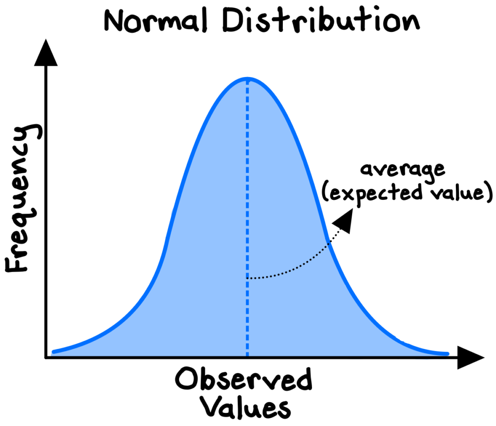
The probability distribution of a random variable defined by a standard bell-shaped curve is known as the normal distribution, which has a meaningful central average (or “mean”) and increasingly rare deviations from the mean. It is a symmetrical distribution in which we expect any random observation to be equally like to fall below or above the average.
Many variables in the real world are normally distributed, or approximately so. A few well-known examples include human height, birth weight, bone density, cognitive skill, job satisfaction, and SAT scores.1
The normal distribution is one of the most powerful statistical concepts to understand, as the properties of normally distributed processes can be modeled and analyzed with well-established statistical methods and readily available software. These tools allow us to make judgments, inferences, and predictions based on data and to quantify the risk around our hypotheses.
If we are not careful, however, the normal model can lead us into grave errors (including the 2008 financial crisis, which we will explore). But first, we should note that although normally distributed phenomena are common in nature, many processes, especially those taking place in complex systems (such as economies), follow distinctly non-normal distributions and often feature a long right-hand “tail” (such as the distribution of individual incomes). We cannot just blindly use the normal model without understanding the distribution of the underlying data and adjusting if necessary.2
However, that is not the full story.
Bells on bells on bells
The normal model is not, in fact, limited to use only with underlying data that is normally distributed.
Consider a set of source data of 1,000 flips of a coin, where heads and tails each occurred exactly 500 times (as we would expect from a fair coin). This data is clearly not normally distributed (see below). So, are the typical statistical tools useless?
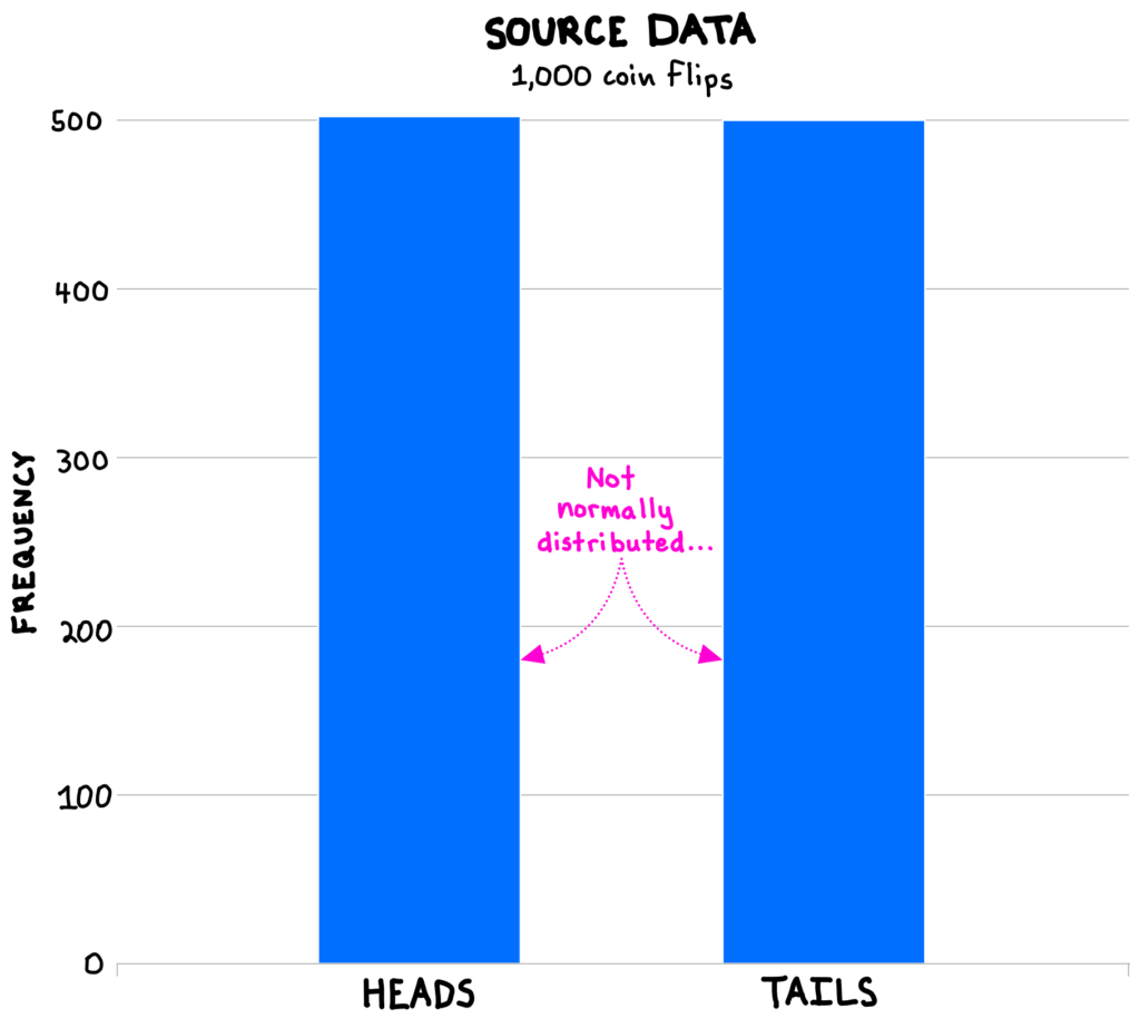
The answer is no.
To see why, let’s take a random sample of, say, 100 flips from the source data, and calculate the fraction of flips that are heads (the sample mean). We expect this percentage to be 50% because that is the population mean of the source data, but, of course, there will be random variation in our sample such that not every sample mean will be exactly 50%.
If we continue to take random samples of 100 flips—say, 500 such samples—and plot the distribution of all the sample means, the distribution of the sample averages will be approximately normal, even though the underlying population data is not normal! This phenomenon is known as the central limit theorem.
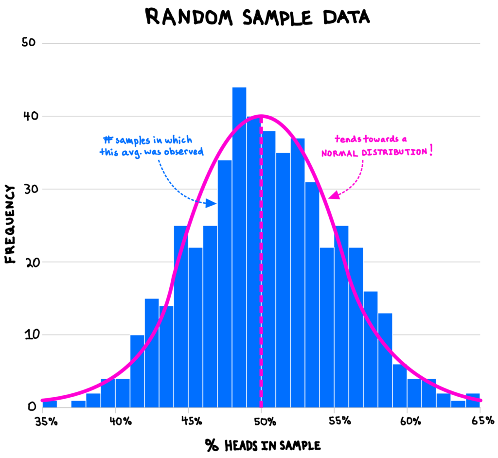
Incredibly powerful in statistics, this maxim explains why bell-shaped distributions are so useful, even though source data sets are rarely perfectly normally distributed: the sample means of just about any process subject to some degree of randomness are eventually normally distributed. This occurs because observed data often represent the accumulation of many small factors, such as how our physical traits (e.g., height, birth weight) emerge from the results of millions of random “copy” operations from our parents’ DNA.3
The central limit theorem enables a wide range of statistical analysis and inference, allowing us to ground our decision making in a solid mathematical foundation.
A truly significant bell
The twin tools of random sampling and statistical analysis using the normal model are widely used and remarkably handy.
Perhaps most significantly, the normal distribution lies at the heart of the scientific method. Because we expect that the observed effects in, say, a clinical trial for a new drug (or any scientific experiment) will tend towards a normal distribution, we can assess how “significant” our observed results are by estimating the probability of observing an outcome that extreme if our drug actually had no effect (the “p-value”). If the normal model tells us that the p-value is very low (say, below 5%), then our trial provides statistically significant support for the drug’s effectiveness.
Manufacturers and engineers use the normal model to set control limits for evaluating some measure of system performance. Observations falling outside the control limits alert the system owner that there could be a problem, since we should expect, under the normal model, that such extreme observations are exceedingly unlikely if the system were functioning normally. We should be thankful that these types of controls exist whenever we board a plane or buy a car.
The normal model should also ring a bell (pun intended…) every time we see the results of a political poll. Attached to the headline poll result should be a “margin of error” which describes the amount of potential error expected around those results, given that random sampling involves variation that follows a normal distribution. For example, a poll might show that the Republican candidate has 48% support in polls, with a margin of error of plus-or-minus 3%, implying the “true” value could be anywhere between 45% to 51%.4
2008 was not normal
Financial institutions and regulators rely heavily on applications of the normal distribution through value at risk (“VAR”) models, which they use to quantify financial risk exposure, establish tolerable risk levels, and assess whether there is cause for alarm.
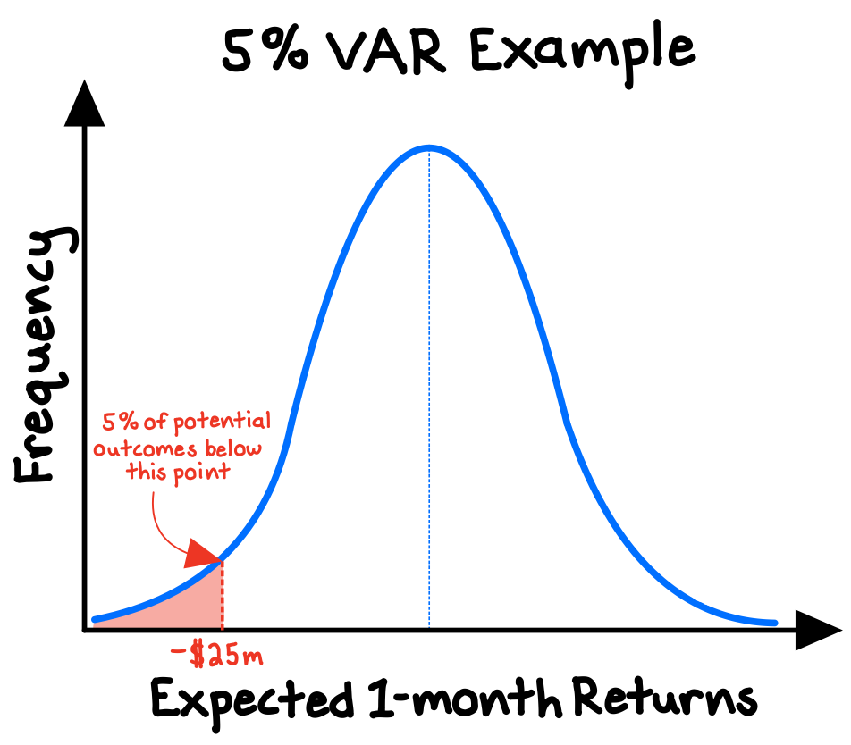
VAR models provide an estimate of the minimum financial losses that should be expected to occur some percentage of the time over a certain time period. For example, an investment firm might estimate that, given an assumed (normal) distribution of their portfolio’s potential returns over the next month, they should expect a 5% probability that they will suffer losses of at least $25m (the “value at risk”).5
The VAR is simply a point on the (assumed) probability distribution of potential returns for a portfolio. The more radical the deviation from today’s conditions, the lower the probability of that outcome—as the normal model would suggest.
VAR supplies a simple, single risk metric that is widely accepted by leading institutions. However, the VAR model also provides an excellent example of the limitations of the normal model—an indeed of models more generally.
Drawing from historical data, the VAR makes strong assumptions about potential future returns, assumptions which are susceptible to error, bias, and manipulation. Moreover, VAR’s use of a normal distribution makes it inadequate for capturing risks of extreme magnitude but low probability, such as unprecedented asset price bubbles or the collapse of the national housing market.
In the aftermath of the 2008 financial crisis, the U.S. House of Representatives concluded that rampant misuse of the VAR model by financial institutions justified excessive risk-taking, which led to hundreds of billions in losses and helped fuel a global recession.6
***
Fluency with basic statistical tools such as the normal model can provide us a valuable edge in our decision-making. It can help us interpret experimental results and political polls, implement quality and safety standards, and quantify financial risks.
But the normal distribution, like all models, is a flawed simplification. It cannot give us certain truth, only suggestions and approximations based on layers of assumptions and theory. Equally important to knowing how to use the normal model is knowing how to determine whether it is appropriate to use in the first place!
References
- Spiegelhalter, D. (2021). The Art of Statistics. Basic Books. 85-91.
- Stine, R., & Foster, D. (2014). The Normal Probability Model. In Statistics for Business: Decision Making and Analysis (2nd ed.). Pearson Education. 307-313.
- Stine, R., & Foster, D. (2014). 297-298.
- Mercer, A. (2016, September 8). 5 key things to know about the margin of error in election polls. Pew Research Center.
- Chance, D., & McCarthy Beck, M. (2023). Measuring and Managing Market Risk. CFA Institute. 2-5.
- U.S. House, Subcommittee on Investigations and Oversight, Committee on Science and Technology. (2009, September 10). The Risks of Financial Modeling: VAR and the Economic Meltdown [H.R. 111-48 from 111th Cong., 1st sess.]. 3-5.